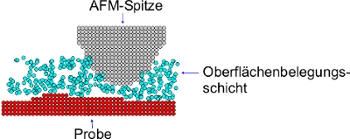
Coarse sketch of the size relation at a low surface contamination,
tip radius app. 1-2 nm

With an Atomic Force Microscope it is possible to image the topography of the top atomic layer. The sketch to the right should give an impression of the size relationships and shows an ultra sharp AFM tip with a tip radius of 1 - 2 nm. In air, any surface is covered with an adsorption layer, the atoms and molecules of which are more or less strongly bound to the surface. When scanning in air, the AFM tip "stirs" this layer. The thickness may be a few nm, however, it often amounts to some hundred nm. In the latter case this is especially disturbing for the most used AC or non-contact mode, where it causes a strong damping of the cantilever oscillation when the tip is close to the surface. One will then get a distorted image that has very little to do with the real surface topography. The viscosity of this surface layer is of great importance; at higher viscosities, even a thin layer may strongly influence the measurement, whereas at lower viscosities the adsorption layer is hardly noticeable.

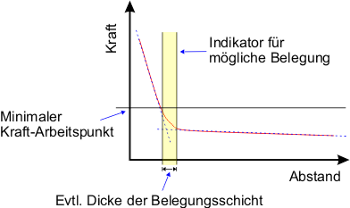
Force-Distance curve as indication of a possible surface contamination

The good thing is that it is possible with the AFM to determine whether or not such a contamination problem exists. For this purpose, one can record a so-called Force-Distance curve (see the sketch to the right).

The distance between the AFM tip and the sample is varied, and the resulting force on the cantilever is measured (via the oscillation in AC mode or via the bending in DC mode). Already when the cantilever is relatively far from the sample surface, it is possible in AC mode to see a slight distance dependency of the damping. This is most due to the air column oscillating between the cantilever and the sample surface. At certain oscillation frequencies you may even determine resonance like conditions; the damping oscillates with a period somewhere in the micro meter scale. In DC mode such effects are not seen. When the cantilever approaches the surface, from a certain point the force will increase strongly. The increase is almost linear. If one specifies a force working point (Force-Setpoint) anywhere within this linear region, one will get a good topography image. The area of interest is the area where the curve goes from the flat part into the linear increase. This transition point is more or less sharp and the width of the transition (yellow in the sketch) is an indication of a possible surface contamination. Generally speaking: the sharper this transition area, the less contaminated is the sample. However, other effects may also result in a deviation from the ideal bend, e.g. discontinuities in the resonance conditions for the cantilever, thus the reverse conclusion is not possible right away. A concrete answer can only be found through a comparison with an "uncontaminated" sample.

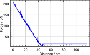
Force-Distance Curve - sample with little contamination

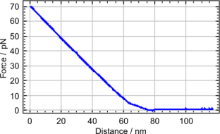
>Force-Distance Curve - sample with contamination
(Thin layer, but high viscosity)

The two diagrams to the right show two measured Force-Distance curves. In the upper curve, the transition layer between the flat part and the strong increase is around 5 nm, and in the lower curve around 15 nm. This is an indication of a contamination layer of the order of magnitude of 10 nm (in a way a low limit for the thickness).

In some case, instead of a Force-Distance curve you may get a simple straight line with an only slight increase towards the sample surface. Most often, this happens when you observe that a scanning does not result in an image of the surface. In AC mode, there are two possible reasons: Either the force measurement does not work, as e.g. when a wrong oscillation peak was used, or the contamination layer is so thick that the force needed to press the cantilever into the contamination layer is higher than the force which totally dampens the oscillation. If such an effect occurs in DC mode, the cantilever may be lose, the laser sport may be located incorrectly, or similar.

Another problem with measuring the contamination layer is that one cannot know whether the layer is on the sample or on the probe tip. A scan over a contaminated sample will collect some of the surface contamination which will hang on to the probe tip, possibly making this unusable. Therefore, before scanning an unknown sample one should make sure that the sample surface is in a defined condition. But one should still be careful! An incorrect cleaning of the sample will often make it more contaminated than before or will ruin the surface. It often helps to flush with ethanol (or better methanol), but this should never be left to dry, rather it should be blown off with a clean gas (e.g. nitrogen). Most often, acetone will also leave a surface contamination layer, so this should be used for the primary cleaning and should be followed by a flushing with alcohol. In all cases, one should use clean reagents (p.a. or better, ultra pure water) and make sure that all holders and vessels are clean. For many samples, a short annealing (heating to 400 °C for 1 minute in a protective gas) is excellent to remove a surface contamination layer, often consisting of watery components. Contaminated cantilevers may be cleaned in the same way. Aggressive cleaning solutions are hydrogen peroxide with hydrocloric acid or ammonia, mixed 50:50 with water. These are especially good at cleaning glass surfaces.

But the best cleaning is always removing the upper layer(s), e.g. by etching. Test samples are also available which in principle are extremely easy to examine, e.g. Highly Oriented Pyrolytic Graphite (HOPG), in which an atomically clean surface can be obtained by removing a surface layer with a piece of adhesive tape.